

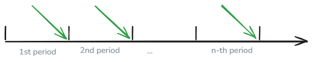
The key difference between an annuity immediate and an annuity due is the timing of payments. In an annuity immediate, payments are made at the end of each period, whereas in an annuity due, payments are made at the beginning of each period.
The term "immediate" might seem misleading since it suggests something paid right away. However, the name comes from a comparison with deferred annuities, which begin payments only after a delay of several periods.
It's also important to distinguish between annuities and life annuities. Regular annuities provide payments for a fixed period, regardless of survival. In contrast, life annuities continue payments only while the policyholder is alive.
Term annuities are denoted as \( \require{enclose} a_{\enclose{actuarial}{n}} \), while term life annuities are written as \( \require{enclose} a^{}_{x:} {}^{}_{\enclose{actuarial}{n}} \). The difference is the \( x \), which represents the age of the policyholder.
In this post, we will focus on regular financial annuities, not life annuities.
Annuity immediate
An annuity immediate is a series of payments made at the end of each period.
Present value
The present value of an annuity immediate, assuming payments of \( 1 \) per period, is calculated as:
\( \begin{aligned} \require{enclose} a_{\enclose{actuarial}{n}} &= \sum_{k=1}^{n} v^{k} \\ &= v + v^{2} + ... + v^{n} \\ &= \frac{1-(1+i)^{-n}}{i} \end{aligned} \)where:
- \( v = \frac{1}{1+i} \) is the discount factor,
- \( i \) is the interest rate per period,
- \( n \) is the number of periods.
For example, the present value of receiving 50 per period for 12 periods (e.g. months) at an interest rate of 1% is:
\( 50 \cdot \frac{1-(1+0.01)^{-12}}{0.01} = 562.75\)This means the current value of these future payments is approximately 562.75.
Python implementation
Using the cashflower package, you can model this as follows:
# model.py
@variable()
def annuity_immediate_pv(t):
    if t == 0:
        return annuity_immediate_pv(t+1) * 1/(1 + 0.01)
    elif t < 12:
        return 50 + annuity_immediate_pv(t+1) * 1/(1 + 0.01)
    elif t == 12:
        return 50
    else:
        return 0
Future value
The future value of an annuity immediate, assuming payments of \( 1 \) per period, is calculated as:
\( \begin{aligned} \require{enclose} s_{\enclose{actuarial}{n}} &= \sum_{k=0}^{n-1} (1+i)^{k} \\ &= (1+i)^{n-1} + (1+i)^{n-2} + ... + 1 \\ &= \frac{(1+i)^{n}-1}{i} \end{aligned} \)For example, with payments of 50 per period for 12 periods at an interest rate of 1%, the future value is:
\( 50 \cdot \frac{(1+0.01)^{12}-1}{0.01} = 634.13 \)This is the amount accumulated after all payments are made, including interest.
Python implementation
You can model this in cashflower as follows:
# model.py
@variable()
def annuity_immediate_fv(t):
    if t == 0:
        return 0
    elif t <= 12:
        return 50 + annuity_immediate_fv(t-1) * (1 + 0.01)
    else:
        return annuity_immediate_fv(t-1)
Annuity due
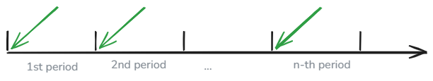
An annuity due is a series of payments made at the beginning of each period.
Present value
The present value of an annuity due, assuming payments of \( 1 \) per period, is calculated as:
\( \begin{aligned} \require{enclose} \ddot{a}_{\enclose{actuarial}{n}} &= \sum_{k=0}^{n-1} v^{k} \\ &= 1 + v + ... + v^{n-1} \\ &= \frac{1-(1+i)^{-n}}{i} \cdot (1+i) \end{aligned} \)Using the same example as before, but with payments at the beginning of each period, the present value is:
\( 50 \cdot \frac{1-(1+0.01)^{-12}}{0.01} \cdot (1+0.01) = 568.38 \)This value is slightly higher than the present value of an annuity immediate because payments are made earlier.
Python implementation
In cashflower, this can be modelled as:
# model.py
@variable()
def annuity_due_pv(t):
    if t < 12:
        return 50 + annuity_due_pv(t+1) * 1/(1 + 0.01)
    else:
        return 0
Future value
The future value of an annuity due, assuming payments of \( 1 \) per period, is given by:
\( \begin{aligned} \require{enclose} \ddot{s}_{\enclose{actuarial}{n}} &= \sum_{k=1}^{n} (1+i)^{k} \\ &= (1+i)^{n} + (1+i)^{n-1} + ... + (1+i) \\ &= \frac{(1+i)^{n}-1}{i} \cdot (1+i) \end{aligned} \)For our example, the future value is:
\( 50 \cdot \frac{(1+0.01)^{12}-1}{0.01} \cdot (1+0.01) = 640.47 \)Since payments are made at the start of each period, each amount accrues interest for an extra period, leading to a higher future value compared to an annuity immediate.
Python implementation
In cashflower, this can be modelled as:# model.py
@variable()
def annuity_due_fv(t):
if t == 0:
return 50
elif t < 12:
return 50 + annuity_due_fv(t-1) * (1 + 0.01)
elif t == 12:
return annuity_due_fv(t-1) * (1 + 0.01)
else:
return annuity_due_fv(t-1)
Relationship between annuity immediate and due
There is a straightforward relationship between an annuity due and an annuity immediate. Since annuity due payments occur one period earlier, their present and future values are always higher by a factor of \( (1+i) \).
Present value relationship
\( \require{enclose} \ddot{a}_{\enclose{actuarial}{n}} \cdot v = \require{enclose} a_{\enclose{actuarial}{n}} \)Applying this to our example:
\( 568.38 \cdot \frac{1}{1+0.01} = 562.75 \)Future value relationship
\( \require{enclose} \ddot{s}_{\enclose{actuarial}{n}} \cdot v = \require{enclose} s_{\enclose{actuarial}{n}} \)For our example:
\( 640.47 \cdot \frac{1}{1+0.01} = 634.13 \)This confirms that an annuity due is simply an annuity immediate shifted one period earlier, leading to a higher present and future value.
In summary, the key difference between an annuity immediate and an annuity due is the timing of the payments. Since annuity due payments occur at the beginning of each period rather than the end, their present and future values are always slightly higher. Understanding this distinction is essential when valuing cash flows in actuarial calculations and financial modelling.
Do you have any questions about annuities or their calculations? Drop them below and let's continue the discussion!
(2025-03-25)
nicely explained, thanks!